4A-6: Calculating Spread and Checking Intake Location

Spread Design Parameters

In this manual, spread (T) refers to the distance from the face of curb to the limit of water on the roadway, while encroachment refers only to how far the water encroaches on the traveled lanes of the roadway. See Figure 1.

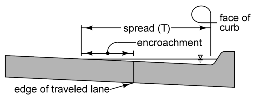
Figure 1: Curb section showing spread and encroachment.

Back to top

Interstates, Freeways, Expressways, and Primary Highways

Table 1 provides maximum allowable encroachment. More stringent requirements may be necessary in areas where encroachment or ponding can result in traffic delays, property damage, or safety concerns such as ice forming in the path of pedestrians.

Back to top

Staged Construction or Detour

Recurrence interval is discussed in Section 4A-5. Use the same encroachment limits as in Table 1.

Back to top

Local Streets

Recurrence interval is discussed in Section 4A-5. Contact the local jurisdiction for encroachment information.

Table 1:  Design storm recurrence interval and allowable encroachment.

situation	design storm recurrence interval	maximum allowable encroachment
Interstates, Freeways, and Expressways
intake on continuous grade	10 year	no encroachment
intake at a sag point	50 year
major storm check	100 year	equivalent of one 12 foot driving lane open to traffic in each direction
Primary Highway (posted speed ≥ 45 mph)
intake on a continuous grade	10 year	no encroachment
intake at a sag point	50 year	3 feet(a)
major storm check	100 year	(b)
Primary Highway (posted speed < 45 mph)
intake on a continuous grade	10 year	3 feet(a)
intake at a sag point	50 year
major storm check	100 year	(b)

⤢

(a) For cross sections with no shoulder, allowable encroachment for two lane roadways is 3 feet onto the traveled lane.  Where there are two or more adjacent lanes in a given direction, allowable encroachment is 6 feet onto the traveled lane in that direction.

(b)The equivalent of one 12 foot lane width open to traffic for two-lane roadways. The equivalent of one 12 foot lane width open to traffic in each direction for three (or more) lane roadways.  Note a lane width could be two partial lanes if they are adjacent and not obstructed.

Back to top

Spread Calculation Procedure

Following is a step-by-step procedure. Explanations and examples are then provided.

Use the Rational Method (Section 4A-5) to find the design storm peak rate of runoff (Q) from each drainage area.  Start at the upstream end and follow the steps below for each area:

1. Calculate the total flow rate to the intake.

2. Calculate the design storm spread (T) to determine how much water is encroaching on the roadway.

3. Use the calculated spread to determine whether the preliminary intake locations are appropriate for the design event. If spread exceeds maximum allowable for the minor design storm, adjust intakes and recalculate Q and spread as required.

Once intake locations are established meeting maximum allowable spread for the minor design storm, evaluate spread for the major design storm.

1. Calculate Q and spread for the major design storm.

2. Evaluate intake locations for the major design storm.  Also evaluate overland flow paths to determine where the water will go when it overtops the curb or crown of the roadway.

 

 

Attention Required

	Spread at sag locations for curb-opening intakes and grate intakes is discussed in Sections 4A-7 and 4A-8 respectively.

⤢

Back to top

Calculation of Total Flow Rate

\(Q = Q_{bp} + Q_{a}\)   (Equation 4A-6_1)

Where,

Q  =   Total flow rate, \(ft^3\)/s.

\(Q_{bp}\)= Bypass flow (flow not intercepted by the upstream intake), \(ft^3\)/s

\(Q_a\)= Flow from the drainage area after the upstream intake, \(ft^3\).

Spread Geometry and Calculations

A curb and gutter combination forms a triangular channel that can carry runoff without interrupting traffic. Spread for a given peak flow (Q) value depends on the type of gutter section used: triangle or multi-triangle.

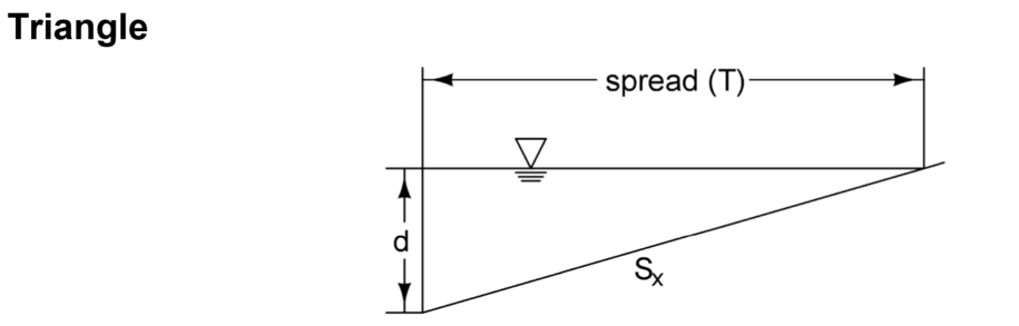
In Figure 2, d is the depth of water at the curb for a spread of T and \(S_X\) is the pavement cross slope.  The spread could include part of a shoulder or traveled lane.  The Triangle section has the assumption that the pavement cross slope under the width of spread is constant.  When the spread is known, the depth of water in the gutter at the curb (see Figure 2) can be calculated:

d = T × \(S_x\), feet (Equation 4A-6_2).

where:

d = Depth at curb for allowable spread, feet (see Figure 4).

T = Spread, feet.

\(S_x\)= Pavement cross slope, ft/ft.

Manning’s equation (modified for triangular gutter flow) is used to determine gutter flow:

\(Q = \frac{K_u}{n} S_x^{1.67} T^{2.67} \sqrt{S_L}\)  (Equation 4A-6_3)

Where,

T    =   Spread, feet.

Q    =   Total gutter flow, \(ft^3\)/s.

\(K_U\) = 0.56

n = Manning’s coefficient (see Table 2).

\(S_x\) = Cross slope of gutter, ft/ft (Note: this is often steeper than the cross slope of the traveled lanes).

\(S_L\) = Longitudinal slope of the gutter, ft/ft.

*For gutters with small slope, where sediment may accumulate, evaluate width of spread by increasing the above values of  “n” by 0.02.

\(T = \left[ \frac{nQ}{K_u S_x^{1.67} \sqrt{S_L}} \right]^{0.375}\)  (Equation 4A-6_4)

The designer should be aware of how selection of a variable affects results.  For example, using a larger n value to account for potential future sediment or older pavement will result in a smaller Q value in Equation 4A-6_3 and a larger T value in Equation 4A-6_4.  Thus, using a larger n value will be conservative with respect to width of spread determinations; however, it will be less conservative with respect to inlet and pipe sizing.

Example Problem 4A-6_1, Calculating Spread (Simple Triangle)

Multi-triangle (Composite Section)

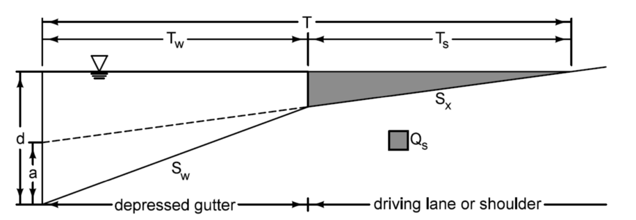
A multi-triangle (depressed) section is more complicated than the simple triangle section and requires different calculations. For calculating spread in a depressed gutter section, use the following formula:

\(T = T_w + T_s\)  (Equation 4A-6_5)

Where,

T = Spread, feet.

\(T_w\)= Depressed gutter section spread, feet.

\(T_s\)= Spread outside of the depressed gutter section, feet.  Ts is calculated as follows:

\(T_s = \frac{T_w \left(\frac{S_w}{S_x}\right)}{\left[\frac{\frac{S_w}{S_x}}{\frac{Q}{(Q - Q_s)} - 1} + 1\right]^{-0.375} - 1}\)   (Equation 4A-6_6)

Where,

Q = Total gutter flow, \(ft^3\)/s.

\(Q_s\)= Flow outside of the depressed gutter section, \(ft^3\)/s.

\(S_x\)= Cross slope of driving lane, ft/ft.

\(S_w\)= Cross slope of depressed gutter, ft/ft. \(S_w\) is determined as follows:

\(S_x = S_x + \frac{a}{12T_x}\)

where a is the depth of the depressed gutter section in inches (see Figure 3).

Example Problem 4A-6_2, Calculating Spread (Multi-Triangle)

Checking Intake Locations

After calculating spread:

1. Compare calculated spread to the allowable spread.

2. If spread exceeds allowable limits, relocate or resize the intake, or add an additional intake.

3. If relocating an intake, recalculate Q for the new drainage area(s) and calculate new values of spread.

4. Repeat the procedure of relocating and adding intakes until spread is within acceptable limits.

Example Problem 4A-6_3, Intake Location Check

Locating Flanking Intakes

On major highways, interstates, freeways, and other roadways on the National Highway System, flanking intakes are required on each side of sag intakes. Flanking intakes function to:

1. Pick up silt before the velocity in the gutter becomes too slow.

2. Reduce ponding at the low point if volumes of water are high or if the intake at the low point becomes plugged.

Flanking intakes are to act in relief, not to intercept flow in order to reduce bypass flow. Therefore, do not include the effects of flanking intakes when sizing and spacing other intakes.

Flanking intakes should be located so each will receive half of the flow should the sag intake become clogged. They should do this before spread at the sag intake exceeds allowable minor design storm spread.  If SW-507 or SW-508 intakes are used as flanking intakes, locate them at an elevation of 0.17d above the sag intake, where d is the depth at curb for the maximum allowable spread.  If SW-509 or SW-510 intakes are used, locate them at an elevation of 0.37d above the sag intake.  When barrier grate intakes (SW-547, SW-548, and SW-549) are being used, locate flanking intakes at an elevation of 0.37d above the sag intake. Refer to Sections 4A-7 and 4A-8 for information on determining d for sag intakes.

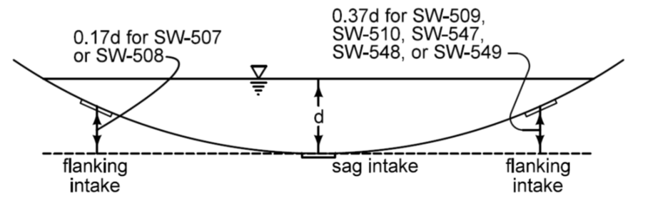
Figure 4:  Locating flanking intakes for a sag intake.

Urban areas can present challenges when locating flanking intakes.  Designers may not be able to properly locate flanking intakes without placing them in intersections with side streets or driveways.  In addition, speeds in urban areas are lower, which allows for higher K values for vertical curves.  As a result, locating a flanking intake at the proper elevation may result in the intake being placed too close to the sag intake.  For situations such as these, designers will need to explore alternatives or obtain a design exception to exclude flanking intakes.

Additional Considerations

HEC-22 discusses additional typical gutter sections, shallow swales, and intake spacing design and provides several examples.

Example Problem 4A-6_1, Calculating Spread (Simple Triangle) 

Calculate the spread (T) for a simple triangular gutter section.

Given:

Empirical Coefficient: \(K_u\) = 0.56.

Cross Slope: \(S_x\)= 0.03 ft/ft.

Manning’s coefficient: n = 0.016 (PC pavement with broom finish).

Total Flow Rate: Q = 1.6 \(ft^3\)/s.

Longitudinal Slope: SL = 0.02 ft/ft.

From Equation 4A-6_4, calculate spread (T): 

Discussion:

Note the curb and gutter unit is often not broom finished and the curb/gutter width (non-broomed area) may carry a substantial amount of the flow, therefore this n value could be too high, but will result in a conservative (possibly higher) T.  When estimating Q, a higher n value is less conservative.

Example Problem 4A-6_2, Calculating Spread (Multi-Triangle) 

Determine Spread (T) for a multi-triangle depressed gutter section.

Given:

      PC Pavement = 31 foot back-to-back.

      Depressed gutter section: \(T_w\) = 3 feet.

      Cross slope of depressed gutter: \(S_w\) = 0.045 ft/ft.

      Cross slope of driving lane: \(S_X\)= 0.020 ft/ft.

      Manning’s coefficient: n = 0.016.

      Total gutter flow: Q = 2.4 \(ft^3\)/s.

      Longitudinal grade: \(S_L\) = 0.005 ft/ft.

      Empirical Coefficient: \(K_u\) = 0.56.

Calculate the spread (T).

Solution:

1. Since the flow outside the depressed gutter section (\(Q_s\)) and spread (T) are unknowns, a trial and error process is required. First, determine the spread using Equation 4A-6_4 and assuming that all the flow will take place in the depressed section of the gutter. Use \(S_w\) for cross slope. 

   \(T = \left[ \frac{nQ}{K_u\, S_w^{1.67}\, \sqrt{S_L}} \right]^{-0.375} = \left[ \frac{0.016 \times 2.4}{0.56 \times 0.045^{1.67} \sqrt{0.005}} \right]^{-0.375} = 6.89\ \text{feet}\)

The spread (T) is more than the 3 foot depressed gutter section (\(T_w\)). Therefore, a multi-triangle section is involved. 

2.  Make an initial estimate of the flow outside of the depressed gutter section (\(Q_s\)). Try \(Q_s\) = 0.60 \(ft^3\)/s. Use Equation 4A-6_6 to calculate spread outside of the depressed gutter section:

   \(T_s = \frac{T_w \times \frac{S_w}{S_x}}        {\left[\frac{\frac{S_w}{S_x}}        {\frac{Q}{(Q - Q_s)} - 1} + 1\right]^{-1}}^{0.375} = \frac{3 \times \frac{0.045}{0.020}}        {\left[\frac{\frac{0.045}{0.020}}        {\frac{2.4}{(2.4 - 0.60)} - 1} + 1\right]^{-1}}^{0.375} = 5.84\ \text{feet}\)

3. Use Equation 4A-6_3 to solve for \(Q_s\) using \(T_s\):

   \(Q_s = \frac{K_u}{n}\, S_x^{1.67}\, T_s^{2.67}\, \sqrt{S_L} = \frac{0.56}{0.016}\, 0.020^{1.67}\, 5.84^{2.67}\, \sqrt{0.005} = 0.40\ \text{ft}^3/\text{s}\)

   If the estimated \(Q_s\) is within 5% of the calculated \(Q_s\) then \(T=T_w+T_s\). If not, try another estimate for Qs and repeat the process. 

4. In this example the calculated \(Q_s\) differs from the estimated \(Q_s\) by more than 5%. Try  = 0.8 ft3/s and use Equation 4A-6_6 to calculate spread outside of the depressed gutter section:

   \(T_s = \frac{T_w \times \frac{S_w}{S_x}}        {\left[\frac{\frac{S_w}{S_x}}        {\frac{Q}{(Q - Q_s)}} + 1\right]^{-1}}^{0.375} - 1 = \frac{3 \times \frac{0.045}{0.020}}        {\left[\frac{\frac{0.045}{0.020}}        {\frac{2.4}{(2.4 - 0.80)}} + 1\right]^{-1}}^{0.375} - 1 = 7.54\ \text{feet}\)

5. Use Equation 4A-6_3 to solve for \(Q_s\) using \(T_s\):

   \(Q_s = \frac{K_u}{n}\, S_x^{1.67}\, T_s^{2.67}\, \sqrt{S_L} = \frac{0.56}{0.016}\, 0.020^{1.67}\, 7.54^{2.67}\, \sqrt{0.005} = 0.79\ \text{ft}^3/\text{s}\)

   The calculated Qs is less than 5% from the estimated Qs. 

6. Use Equation 4A-6_5 to calculate spread:

   \(T = T_x + T_s = 3 + 7.54 = 10.54\ \text{feet}\)

   ---

Example Problem 4A-6_3, Intake Location Check

Given:

The preliminary location analysis for two intakes places them 300 feet apart. The longitudinal gutter slope between the intakes is 1.5%. The cross slopes for the roadway and gutter are both 2%. The bypass from the first intake is 0.11 \(ft^3/s\) and the peak flow from the drainage area for the second intake is 1.90\(ft^3/s\) . Determine if the downstream intake is appropriately spaced for a maximum allowable spread of 8 feet. Assume n = 0.016.

Determine:

The total flow to the second intake is the bypass flow from the first intake plus the peak flow from the drainage area:

\(Q = Q_{bp} + Q_a = 0.11 + 1.90 = 2.01\ \text{ft}^3/\text{s}\)

Use Equation 4A-6_4 to determine spread:

\(T = \left[\frac{nQ}{K_u\, S_x^{1.67}\, \sqrt{S_L}}\right]^{-0.375} = \left[\frac{0.016 \times 2.01}{0.56 \times 0.02^{1.67} \sqrt{0.015}}\right]^{-0.375} = 8.72\ \text{feet}\)

This exceeds the maximum allowable spread of 8 feet. Two options are available:

1. Relocate the second intake closer to the first intake to reduce the drainage area flowing into the second intake.
2. Resize the upstream intake to reduce bypass.

Locating Flanking Intakes for a Sag Intake

Flanking intakes should be located so each intake intercepts half of the flow to the sag intake should the sag intake become completely clogged, see the figure below.  The locations are determined by calculating the depth required at the flanking intake (df) to intercept half of flow intercepted by the sag intake. 

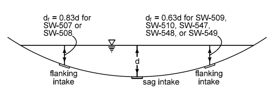
For this, the intakes are assumed to be in weir flow.  The equation to determine the depth of flow is (assuming an intake with a depression, see Section 4A-7 for more information):

\(d = \left[\frac{Q}{2.3\, (L + 3.6)}\right]^{0.67}\)

where:

d = Depth of ponding at maximum allowable spread for the minor storm.

Q = Intercepted flow, \(ft^3/s\) (\(m^3/s\)).

L = Length of throat opening.

For an SW-509 or SW-510, L = 8 feet, so:

\(d = \left[\frac{Q}{2.3\, (8 + 3.6)}\right]^{0.67} = 0.1108\, Q^{0.67}\)

SW-507 or SW-508 is used as Flanking Intake

If an SW-507 or SW-508 is used, L = 4 feet.  The depth at the flanking intake (\(d_f\)) required to intercept 0.5Q is:

\(d_f = \left[\frac{0.5Q}{2.3\,(L + 3.6)}\right]^{0.67} = \left[\frac{0.5Q}{2.3\,(4 + 3.6)}\right]^{0.67} = 0.0924\,Q^{0.67} \approx 0.83 \times 0.1108\,Q^{0.67} = 0.83d\)

This means the flanking intakes should be located at an elevation of (1 – 0.83)d above the sag intake.

SW-509 or SW-510 is used as Flanking Intake

If an SW-509 or SW-510 is used as a flanking intake, the depth at the flanking intake (\(d_f\)) required to intercept 0.5Q is:

\(d_f = 0.1108\,(0.5Q)^{0.67} = 0.5^{0.67} \times 0.1108\,Q^{0.67} = 0.63d\)

This means the flanking intakes should be located at an elevation of (1 – 0.63)d above the sag intake.

SW-547, SW-548, and SW-549 Barrier Grate Intakes

When SW-547, SW-548, or SW-549 barrier grate intakes are being used, the flanking intake will be the same size as the sag intake.  This is similar to the situation above for SW-509 or SW-510 being used as flanking intakes.  As a result, flanking intakes are located in the same manner: (1 – 0.63)d above the sag intake.

Tips for Determining Preliminary Intake Spacing and Drainage Areas

 If the majority of a drainage area is pavement (Figure 1), the following instructions will help determine the preliminary spacing of intakes.

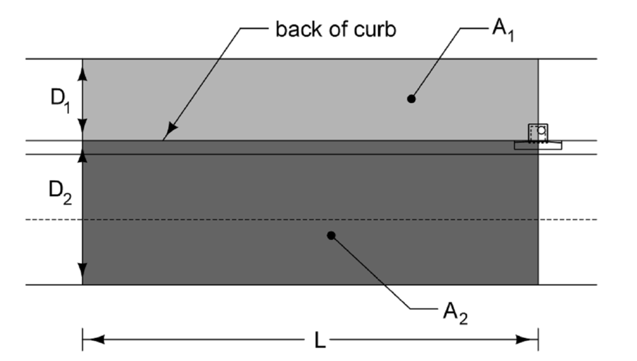
1.  Calculate maximum allowable Q based on maximum allowable width of spread:

\(Q = \frac{K_u}{n}\, S_x^{1.67}\, T^{2.67}\, \sqrt{S_L}\)   (Equation 3)

where:

         Q  =  gutter flow rate, \(ft^3/s\).

         \(K_u\)  = empirical coefficient equal to 0.56.

         n   =  Manning’s roughness coefficient.  See Table 6, Section 4A-5.

\(S_x\) = gutter cross slope, ft/ft. 

         T   =  maximum allowable spread, feet.  See Table 1.

         \(S_L\) =  longitudinal gutter slope, ft/ft.

2. Estimate Intensity (I).  Assume a \(T_c\) = 5 minutes. Use Table 2 or Table 3 of Section 4A-5 to find the corresponding intensity value (I) for the appropriate Region.

3. Calculate the preliminary intake spacing (L):

   \(L = \frac{43{,}560 \times Q}{I\,(C_1D_1 + C_2D_2)}\)

   where,

      L, \(D_1\), and \(D_2\) are in feet and I is in in/hr

   The equations for L are derived as follows:

   \(A_1 = \frac{D_1 \times L}{43{,}560} \qquad A_2 = \frac{D_2 \times L}{43{,}560}\)   (Where A1 and A2 are in acres)

   For the composite area= \(C = \frac{C_1A_1 + C_2A_2}{A_1 + A_2}\)

   where:

   \(C_1\) and \(C_2\) are the imperviousness coefficients for areas \(A_1\) and \(A_2\). See Table 1, Section 4A-5.

   From the Rational equation:

   \(Q = CIA = \frac{C_1A_1 + C_2A_2}{A_1 + A_2}\, I\, (A_1 + A_2) = \left[C_1 \frac{D_1 L}{43{,}560} + C_2 \frac{D_2 L}{43{,}560}\right] I = \frac{(C_1D_1 + C_2D_2)\, LI}{43{,}560}\)

   Solving for L:

   \(L = \frac{43{,}560 \times Q}{I(C_1D_1 + C_2D_2)}\)

   where:

    L, \(D_1\), and \(D_2\) are in feet and I is in in/hr

    

Chronology of Changes