
Content Information
On this page...
The Rational Method
For most roadway stormwater drainage systems, the Rational Method can be used to determine peak flow (Q). If drainage areas involve pump stations or include topography or structures that retain or detain water, the Rational Method cannot be used. Use other nationally accepted methods.
The Rational Method is limited to drainage basins 160 acres or smaller. This is a result of the assumptions associated with the Rational Method, which include:
Recurrence interval (TR) used for estimating peak flow is the same as that for determining rainfall intensity (i.e., a 50 year storm is assumed to produce a 50 year peak flow). Peak flow is assumed to occur when the entire watershed is contributing to flow.
Rainfall intensity is the same over the entire drainage area and is uniform over a time duration equal to the time of concentration (Tc).
For drainage areas larger than 160 acres, other methods of determining peak flow (for example, the SCS (NCRS) peak flow method) are required. These are discussed in HEC-22.
The Rational Equation
The Rational Method uses the Rational equation given below:
Q = CIA (Equation 4A-5_1)
where:
Q = Peak flow, ft3/s.
C = Runoff coefficient (dimensionless).
I = Rainfall intensity, in/hr.
A = Drainage area, acres.
Back to topDrainage Area (A)
A drainage basin, or watershed, consists of all drainage areas that contribute flow to an outlet. A drainage basin may consist of one or several drainage areas.
For stormwater system design, a drainage area (A) is the combined area of all surfaces that drain to a given location such as a swale, intake or culvert inlet, pond, stream, etc. Following are some questions to investigate when evaluating a drainage area. Local maintenance authorities may be able to provide information. Documentation of the investigation is important:
How are individual lots graded? Rear to front? Half to the rear and the other half to the front?
Will existing contour lines remain the same, or are there known intentions for the area be regraded?
Which direction will water flow down the gutters of the streets?
At intersections, what direction will bypass flow or ponded flow go? Will water flow around the corner or flow across the intersection?
Will water run the same direction for all design rainfall intensities? Does bypass flow drain to the same downstream location as the underground storm sewer pipe?
Are there known or expected roof drains, tile drains, subdrains, sump pumps, or other items that drain to the system? Are some of these draining water from other drainage basins?
Section 4A-2 lists sources that may be useful when examining drainage areas.
Back to topRunoff Coefficient (C)
The runoff coefficient (C), also called the “coefficient of imperviousness,” is the ratio of runoff to rainfall. Factors that contribute to C include:
Shape of the drainage area.
Slope of the watershed.
Land use (percentage of impervious surface and surface type).
Character of the soil.
Basin storage potential (potholes, roof storage, etc.).
Previous (antecedent) moisture conditions.
Interception by vegetation or animal life (e.g. a beaver dam).
Rainfall duration.
Rainfall intensity.
Recurrence interval (rainfall frequency).
Runoff coefficient values for 5 year, 10 year, 50 year, and 100 year recurrence intervals are given in Table 1.
Table 1: Runoff coefficients for the Rational Method.
If future land use is unknown, the runoff coefficient should be conservatively based.
Occasionally a single C value can adequately describe an entire project or area. Typically, a different C value is required for each inlet and composite C values are often required. When a drainage area is composed of more than one distinct part, use the weighted average equation below to find a composite C.
\(C = \frac{C_1A_1 + C_2A_2 + C_3A_3 + \ldots + C_nA_n}{A_1 + A_2 + A_3 + \ldots + A_n}\) (Equation 4A-5_2)
Where:
\(A_1, A_2, A_3, \ldots, A_n\)= areas of the distinct parts.
C1 = C value for A1, C2 = C value for A2, etc.
Example Problem 4A-5_1, Determining Composite C
Back to topRainfall Intensity (I)
Rainfall intensity (I) is the average rate of rainfall given in in/hr that occurs over the duration of a storm. Rainfall intensity is required to use the Rational method. To calculate I, the designer must first select a recurrence interval (TR). Next the designer calculates the time of concentration (Tc). Once TR and Tc are known, I is determined using Table 2 (for the Rational method, storm duration is the same as Tc). Often, Tc falls between the values in the tables, so I needs to be interpolated.
Table 2: Rainfall Intensities (inches/hour) for Recurrence Intervals of 2 to 100 years\(^{1}\) .
* Sectional code (see map)
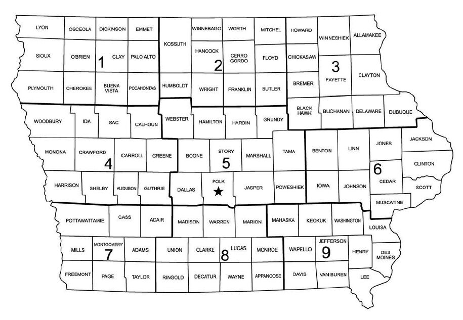
Based on NOAA Atlas 14: Precipitation-Frequency Atlas of the United States, Volume 8 Version 2.0: Midwestern States. National Oceanic and Atmospheric Administration. Rainfall intensities for each climatic section were calculated by averaging the intensities for the counties included in each climatic section.
Rainfall intensity does not account for a rainfall’s variable intensity over time or across a basin, or for how much rainfall fell prior to the period in question. Designers should keep these factors in mind, especially for areas prone to flash flooding.
Back to top
Recurrence Interval (Frequency)
When designing stormwater drainage systems, designers rely on the recurrence interval (TR). Recurrence interval is referred to in a number of different ways: frequency, design flood frequency, storm frequency, recurrence frequency, exceedence interval, or return period.
Recurrence interval is based on probability:
\(T_R = \frac{1}{p}\)
Where,
\(T_R\)= Recurrence Interval in years.
p= Probability of a storm event that equals or exceeds a specified flow occurring in a given year.
Table 3: Recurrence interval and probability.
Since TR is based on probability, a recurrence interval is not the actual interval for which a storm event is expected to occur. Instead, it represents the probability a storm event will occur in any given year. For example, a storm event with a 50 year recurrence interval has a 2% probability of equaling or exceeding a specified flow in any given year. A 50 year storm event may actually occur several times in a 50 year span, several times in one year, or just once in 100 years. When communicating with or relating to the general public, using terms such as “X% Chance Storm Event” may help reduce confusion and concerns.
Designing a stormwater drainage system to handle the worst storm event that could happen would likely be too costly for most situations. On the other hand, designing a system that is overtaxed by even minor storm events can result in flooding that creates safety issues or economic hardships. Since the consequences of flooding in some areas are more severe than in others, desired design TR values vary for different elements of a system depending on the area drained, area conveying the runoff, and the need to avoid flooding. The selection of the design TR is based on several factors, which can include safety, economics, policy, or regulatory requirements. The goal is to balance the cost of the system with potential risk and damage costs.
Interstates, Freeways, Expressways, and Primary Highways
Table 4 provides minimum required design TR values for interstates, freeways, expressways, and primary highways. More stringent requirements (higher design recurrence intervals) may be necessary in areas where encroachment or ponding can result in traffic delays, property damage, or safety concerns.
Table 4: Required minimum design recurrence interval values
Staged Construction or Detour
Recurrence interval design values selected for staged construction and detours depend on traffic counts, speeds, how long the system will be in place, accommodations for overtopping or bypassed flow, and the consequences should the system be overtaxed. Two years is the minimum recurrence interval design value allowed for temporary staged construction.
Local Streets
Recurrence interval design values for local jurisdictions vary throughout the state. Contact the local jurisdiction.
For reconstruction projects involving storm sewer, existing systems should be analyzed and new systems should be sized using current recurrence intervals even if the original system (and other systems tying into it) was sized using a smaller recurrence interval.
In using the Rational equation to determine peak flow for a given TR (e.g. 10 year), the same TR must be used when determining C and I. Occasionally the contributing drainage area A is affected by the TR as well, due to an increased chance of flow bypassing from one watershed to another during large recurrence interval events.
Back to topTime of Concentration (Tc)
Time of concentration (Tc) is the time required for water falling on the hydraulically most remote point in a drainage area to flow to the point of interest. Remoteness relates to time rather than distance. Factors affecting Tc include:
Surface roughness. Rough terrain, such as undeveloped areas, impedes flow of runoff more than smooth surfaces such as pavement. This increases Tc.
Channel shape and flow patterns. Channels typically convey runoff more efficiently than flat terrain. This reduces Tc.
Slope. The velocity of runoff increases with increase in slope. This reduces Tc.
Water traveling a short distance across rough, flat terrain may require more time to reach a point of interest than water traveling a longer distance across smooth, steep terrain. Thus, the most hydraulically distant point in a drainage area may not be the point located furthest from the point of interest.
Total \(T_C\) may consist of several components and is calculated as follows:
\(T_c = T_{c\,\text{sheet}} + T_{c\,\text{shallow}} + T_{\text{open channel}} \;\) (Equation 4A-5_3)
Where,
\(T_C\)= Total time of concentration, minutes.
\(T_{c\,\text{sheet}}\)= Time of concentration for overland sheet flow, minutes.
\(T_{c\,\text{shallow}}\)= Time of concentration for shallow concentrated flow, minutes.
\(T_{c\,\text{open channel}} = T_{c\,\text{gutter}} + T_{c\,\text{pipe}} + T_{c\,\text{swale}}\)
where,
\(T_{c\,\text{gutter}}\)= Time of concentration for gutter flow, minutes.
\(T_{c\,\text{pipe}}\)= Time of concentration for pipe flow, minutes.
\(T_{c\,\text{swale}}\)= Time of concentration for flow in a swale, minutes
The following worksheet will aid with calculating Tc. The components of the worksheet are further explained below.
Time of Concentration Worksheet (214.08 KB) .pdf
Overland Sheet Flow (\(T_{c\,\text{sheet}}\))
Overland sheet flow is the shallow mass of runoff over plane surfaces (e.g. parking lots, lawns). Overland sheet flow usually occurs over a short distance at the high end of a drainage area. The National Resources Conservation Service (NRCS) recommends limiting overland sheet flow to 100 feet for unpaved areas. This manual follows the recommendation of NRCS. For paved surfaces, the maximum is 300 feet.
Use the kinematic wave equation below to estimate Tc for overland sheet flow:
\(T_{c\,\text{sheet}} = \frac{K_u}{I^{0.4}} \left( \frac{nL}{\sqrt{S}} \right)^{0.6}\) (Equation 4A-5_4)
Where,
\(T_{c\,\text{sheet}}\)= Overland sheet flow travel time, minutes.
\(K_U\)= Empirical coefficient equal to 0.933.
n= Manning’s roughness coefficient for overland flow (see Table 5), based on very shallow flow depths of up to 0.1 feet.
L= Overland flow path length, feet.
I = Rainfall intensity rate, in/hr.
S = Slope of the overland flow path, ft/ft.
Table 5: Manning’s roughness coefficient (n) for overland flow.
Table 2 will be necessary to calculate \(T_{c\,\text{sheet}}\). Since both \(T_C\) and I are unknowns, a trial and error process is required using the rainfall intensity values in Table 2. This is how it works:
Refer to Table 2 to determine which Section code is appropriate. Choose a value from the “duration” column (this serves as \(T_{c\,\text{sheet}}\) ) in Table 2 with the corresponding I from the appropriate “recurrence interval” (10 year or 50 year) column.
Calculate \(T_{c\,\text{sheet}}\) by substituting I into Equation 4A-5_4.
Compare the selected value of \(T_{c\,\text{sheet}}\) with the calculated value from Step 2.
If the value of \(T_{c\,\text{sheet}}\) from Step 2 is less than 5 minutes, use Tc sheet = 5 minutes.
If the selected Tc sheet is within one minute of \(T_{c\,\text{sheet}}\) from Step 2, then \(T_{c\,\text{sheet}}\) equals the selected value.
If the selected \(T_{c\,\text{sheet}}\) is not within one minute of \(T_{c\,\text{sheet}}\) from Step 2, then select another value for \(T_{c\,\text{sheet}}\) (try a value close to the calculated \(T_{c\,\text{sheet}}\)). This may require using values of \(T_{c\,\text{sheet}}\) not in the tables. If this is the case, I will need to be interpolated. This process is demonstrated in the Sheet Flow Example Problem.
Repeat Steps 2 and 3 until the selected value for \(T_{c\,\text{sheet}}\) is within one minute of the calculated \(T_{c\,\text{sheet}}\).
Example Problem 4A-5_2. Overland Sheet Flow
Back to topShallow Concentrated Flow (\(T_{c\,\text{shallow}}\))
After a short distance (depending on ground cover, but always less than 100 feet), overland sheet flow starts to concentrate in rills, and then in gullies. This flow is referred to as shallow concentrated flow. The velocity of this flow is estimated using a relationship between velocity and slope. To calculate \(T_{c\,\text{shallow}}\), first estimate the velocity of flow using the following equation:
\(V = K_u\, k \sqrt{S}\) (Equation 4A-5_5)
Where:
V= Velocity of flow , ft/s
S= Slope , ft/ft. *
k = Intercept coefficient (see Table 6).
\(K_u\)= Units conversion factor*, 33.
*HEC-22 bases slope on percent. Units conversion factors in HEC-22 are smaller by a factor of 10.
Table 6: Intercept coefficients for shallow concentrated flow.
Once velocity has been determined, use the equation below to calculate \(T_{c\,\text{shallow}}\)
\(T_{c\,\text{shallow}} = \frac{L}{60V}\) (Equation 4A-5_6)
Where,
\(T_{c\,\text{shallow}}\)= Shallow concentrated flow travel time, minutes.
L = Flow length, feet.
V = Velocity of flow, ft/s.
Example Problem 4A-5_3, Shallow Concentrated Flow
Open Channel Flow
Open channels for roadway stormwater drainage systems consist of drainage swales, pipes flowing partially full, and gutters.
Gutter Flow (\(T_{c\,\text{gutter}}\))
Flow time for runoff in the gutter is typically small (1 to 2 minutes, or less) compared to the total Tc, and it is often not included. This produces slightly more conservative results for rainfall intensity, which adds in a factor of safety.
For long gutter lengths (several hundred feet), flat gutter slopes (around or less than 0.50%), or low flows (less than 0.50 ft3/s), gutter flow time may be several minutes and may need to be included in total (\(T_C\)). To estimate gutter flow time, first determine the average velocity using one of the equations below:
\(V = \frac{2Q}{T^2 S_x}\) (Equation 4A-5_7, uniform cross section)
\(V = \frac{2Q}{T^2 S_x + W^2 (S_W - S_x)}\) (Equation 4A-5_7, composite gutter section)
where:
Q = Flow in gutter, ft3/s.
T = Spread, feet.
W = Width of depressed section, feet
\(S_x\)= Cross slope of pavement, ft/ft.
\(S_w\)= Cross slope of depressed gutter section, ft/ft.
After calculating velocity, use Equation 4A-5_6 to determine (Tc gutter).
Pipe Flow (\(T_C\) pipe)
Refer to General Information for Pipe Design in Section 4A-10.
Drainage Swales (\(T_{c\,\text{swale}}\))
Use Manning’s equation (Equation 4A-5_8 below) to estimate average flow velocity. The Manning’s roughness coefficient ‘n’ is a function of several parameters including: channel material type, roughness, thickness (such as size of rocks or height of vegetation), flow velocity and flow depth. This coefficient can have a dramatic result in the outcome of the equation. Table 7 provides a brief list of some average ‘n’ values for consideration in the design process. The designer should have a good understanding of how and when to use this equation and how to evaluate the use of an appropriate ‘n’ value before proceeding.
\(V = \frac{K_u}{n} \left( \frac{A}{P_{\text{wetted}}} \right)^{0.67} \sqrt{S}\) (Equation 4A-5_8)
where:
V = Velocity of flow, ft/s.
S = Slope, ft/ft.
n = Manning’s roughness coefficient for open channel flow (See Table 7).
\(K_u\)= Units conversion factor, 1.49.
A = Cross sectional flow area, \(ft^2\).
\(P_{\text{wetted}}\)= Wetted perimeter (surface in contact with water), feet.
Table 7: Values of Manning's coefficient (n) for open channel flow.
After calculating velocity, use Equation 4A-5_5 to determine (\(T_{c\,\text{swale}}\)).
To estimate \(T_{c\,\text{swale}}\), the design flow, Q, is desired to estimate flow depth in order to estimate wetted perimeter (\(P_{\text{wetted}}\)). However, Tc is required to estimate Q; therefore, this is an iterative process that is simplified by hydraulic computer models and spreadsheets. The general design process should be understood before using a model and checking results.
Back to topCalculating Peak Flow (Q) for a Drainage Area
The following example demonstrates the process for determining peak flow for a drainage area.
Example Problem 4a-05_4, Determining Peak Flow Values
Back to topDesign Application
Distinct parts of a drainage area may produce higher peak flows than if a composite ‘C’ value is used for the total drainage area. Each of these parts should be examined individually, as well as in combination, to determine which produces the largest peak flow. When determining Q for the composite area, use the flowpath associated with the longest Tc.
Runoff analysis must consider flow from outside the study area that may enter the site either as surface runoff or as contained flow in tiles and pipes.
In addition to the determination and analysis of existing and proposed design flows for each design event, consideration must be given to interim construction conditions, staged construction, and reconstruction
Interim Construction Conditions
During construction, vegetative cover may be diminished resulting in increased runoff coefficients and peak flows. Proposed design flow determinations may not be adequate to evaluate interim construction conditions (including erosion and sediment control needs).
Inlets are generally protected from sediment by erosion control devices, such as filter socks, which can trap runoff. Evaluate potential ponding and impacts caused by such erosion control devices.
Sediment basins may be desired to both store excess runoff and capture excess sediment.
Staged Construction
Designers occasionally need to select temporary drainage structures to accommodate staged construction. The level of design required must be commensurate with the risks (including traffic, speed, location, etc.) and should be discussed and selected by the design team.
Reconstruction
Generally reconstruction results in replacing or upgrading a storm sewer system. Occasionally the contributing runoff area has been modified either by overland contribution or closed system contribution (from other storm drain systems that have been tapped into the project area system). Quite often design parameters (e.g. design flow) and design coefficients (impervious area) have changed since the original system design. However, don’t reduce the number or size of existing inlets or pipes without significant design evaluation and concurrence from the local and maintenance authorities.
Back to top
Example Problem 4A-5_1: Determining Composite C
Determine the composite C value for the following situation assuming a 10 year (minor storm) recurrence interval.
A drainage area consists of the following:
Residential ¼ acre lots known to be 40% impervious based on roof area, sidewalks, driveways and other impervious areas:
0.18 acres, C = 0.49
Lawn, 1.5% slope known to be 0.0% impervious based on roof areas, sidewalks, and driveways and other impervious areas:
0.25 acres, C = 0.22
Pavement:
0.09 acres of new PCC, C = 0.95
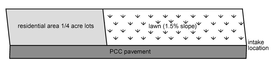
Use Equation 4A-5_2 to determine a composite C:
\(C = \frac{(0.18 \times 0.49) + (0.25 \times 0.22) + (0.09 \times 0.95)}{0.18 + 0.25 + 0.09} = 0.44\)
Another way to look at this, using the same example, is through percent land use. Assume we were given or estimated that 34.6%* of the drainage area is residential lots, 48.1%* is open lots, and 17.3%* is PCC roadway (with the assumptions stated above for all of these). Composite C is calculated as follows:
\(C = \frac{(34.6\% \times 0.49) + (48.1\% \times 0.22) + (17.3\% \times 0.95)}{100\%} = 0.44\)
* Percent values were calculated by dividing the sub area by the total area and multiplying the resultant by 100.
Back to top
Example Problem 4A-5_2, Overland Sheet Flow
Determine (\(T_{c\ \text{sheet}}\) ) for a flow length of 65 feet.
Given:
Average slope: S = 0.02 ft/ft
Manning coefficient: n = 0.24 (well established dense grasses, see Table 6)
Recurrence interval: T = 10 years
Keokuk, Iowa: Section Code = 09 (See Table 2)
Solution:
- Select \(T_{c\ \text{sheet}}\) from Table 2 (a portion is shown below). Start with 10 minutes, which corresponds to an I = 5.62 in/hr
- Use Equation 4A-5_4 with I = 5.62 in/hr to compute \(T_{c\ \text{sheet}}\):
\(T_{c\ \text{sheet}} = \frac{K_u}{I^{0.4}} \left( \frac{nL}{\sqrt{S}} \right)^{0.6} = \frac{0.933}{5.62^{0.4}} \left( \frac{0.24 \times 65}{\sqrt{0.02}} \right)^{0.6} = 7.86\) minutes
- The calculated value of \(T_{c\ \text{sheet}}\) is not within 1 minute of the assumed value of 10 minutes.
- Try value of \(T_{c\ \text{sheet}}\) close to the calculated value. Try \(T_{c\ \text{sheet}}\) = 8 minutes. This falls between 10 minutes and 5 minutes in Table 2, so this will require interpolating for (I).
\(\frac{8 - 10}{5 - 10} = \frac{I - 5.62}{7.68 - 5.62}, \quad I = 5.62 + \frac{8 - 10}{5 - 10}(7.68 - 5.62) = 6.44\) in/hr
Calculate \(T_{c\ \text{sheet}}\) and compare to the assumed value of 8 minutes:
\(T_{c\ \text{sheet}} = \frac{K_u}{I^{0.4}} \left( \frac{nL}{\sqrt{S}} \right)^{0.6} = \frac{0.933}{6.44^{0.4}} \left( \frac{0.24 \times 65}{\sqrt{0.02}} \right)^{0.6}\) = 7.45 minutes
The calculated value and assumed value of Tc sheet are within one minute of each other, so \(T_{c\ \text{sheet}}\) = 8 minutes
Back to top
Example Problem 4A-5_3, Shallow Concentrated Flow
Determine (Tc shallow) for a shallow concentrated flow length of 150 feet.
Given:
\(K_u\) = 33, shallow flow equation conversion factor.
Intercept coefficient: k = 0.457 (grassed waterway, see Table 7).
Flow length: L = 150 feet.
Average slope: S = 2% (0.02 ft/ft).
Recurrence interval: T = 10 years.
Solution:
Use Equations 4A-5_5 & 4A-5_6 to find \(T_{c\ \text{shallow}}\) :
\(V = K_u\, k\, \sqrt{S} = 33 \times 0.457 \sqrt{0.02} = 2.13\) ft/s
\(T_{c\ \text{shallow}} = \frac{L}{60V} = \frac{150}{60 \times 2.13} = 1.2\) minutes ( round to 1 minute )
Discussion:
Round \(T_{c\ \text{shallow}}\) to the nearest minute. If \(T_{c\ \text{shallow}}\) is less than 0.50 minutes,\(T_{c\ \text{shallow}}\) can be ignored.
Back to top
Problem 4A-5_4, Determining Peak Flow Values
Determine the peak flow for a 10 year recurrence interval for an intake located on a Primary Highway with a 31 foot back-to-back pavement (two 12 foot lanes with 3½ foot curb and gutter section using 6 inch curbs).
Location: Jewel, Iowa.
Drainage area consists of the following:
Lawn, 2.5% slope Bermuda grass (no buildings, driveways, or sidewalk areas)
A = 0.25 acres (approximately 40 feet × 265 feet).
C = 0.25 for a 10-year recurrence interval.
Average Slope of Surface, S = 2.5%.
\(T_c\) and I have already been determined to be:
\(T_c\)= 7 minutes. When calculating \(T_c\), time runoff is in the gutter was assumed to be negligible.
I = 6.79 in/hr for a 10 year recurrence interval.
Pavement:
A = 0.09 acres of new PCC (15½ feet × 265 feet). Runoff flows from crown to gutter.
C = 0.95 for a 10 year recurrence interval.
Pavement Cross Slope, \(S_x\) = 2.0%.
Gutter Cross Slope, \(S_w\) = 2.0%.
Length in Gutter = 265 feet.
Longitudinal Slope, \(S_L\) = 1.5%.
Manning’s Coefficient, n = 0.016 .
\(T_c\) and I have already been determined to be:
\(T_c\) = 5 minutes. Actual \(T_c\) was determined to be less than 5 minutes; however, to determine I, a minimum \(T_c\) of 5 minutes is required.
I = 8.10 in/hr for a 10 year recurrence interval.
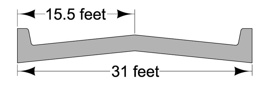
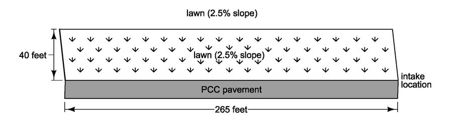
Jewel is located in Section Code 5 (see Table 2 of Section 4A-5).
1) Lawn.
Calculate peak flow using Equation 4A-5_1:
Q = CIA = 0.25 × 6.79 × 0.25 = 0.42 ft3/s
2) Paved area.
Calculate peak flow using Equation 4A-5_1:
Q = CIA = 0.95 × 8.10 × 0.09 = 0.69 ft3/s
3) Combined area.
To calculate peak flow for the combination of the lawn and the paved area, use the flowpath associated with the longest \(T_c\). In this situation, the lawn has the longest \(T_c\) (7 minutes). Use Equation 4A5-2 to calculate a weighted C value.
\(C = \frac{(0.25 \times 0.25) + (0.95 \times 0.09)}{0.25 + 0.09} = 0.44\)
Calculate the peak flow for the combined area (Tc = 7 minutes, so I = 6.79 in/hr):
Q = CIA = 0.44 × 6.79 × (0.25 + 0.09) = 1.02 \(ft^3\)/s.
The combined area produces the largest peak flow. Use this value when determining the final size of the intake.
Back to top
Hydrologic Soil Groups
The Hydrologic Soil Groups, as defined by NRCS soil scientists, are:
Group A - Low runoff potential - Soils having a high infiltration rate even when thoroughly wetted, consisting chiefly of deep, well to excessively-drained sands or gravels.
Group B - Soils having a moderate infiltration rate when thoroughly wetted, and consisting chiefly of moderately deep to deep, moderately well to well-drained soils with moderately fine to moderately coarse texture.
Group C - Soils having a slow infiltration rate when thoroughly wetted, and consisting chiefly of soils with a layer that impedes downward movement of water or soils with moderately fine to fine texture.
Group D - High runoff potential. Soils having a very slow infiltration rate when thoroughly wetted, and consisting chiefly of clay soils with a high swelling potential, soils with a permanent high water table, soils with a clay pan or clay layer at or near the surface, and shallow soils over nearly impervious material.
Back to top
Chronology of Changes
Back to top